Polymer physics, thermodynamics and bioinformatics

TL;DR — We built three separate statistical-physics formulations of protein alignment: a learned pair Hamiltonian with an exact partition function, a free-energy scorer with predicted contact and geometry terms, and a learned pair-HMM. They are independent implementations rather than independent evidence — they share one team, one encoder family, and two structure-derived benchmarks, so a flaw in the representation would show up in all three. Measured against a fixed affine Smith-Waterman verifier on frozen ESM2-8M embeddings, none of them earned their place. The learned neural Hamiltonian tied fixed Smith-Waterman at 14.88x the CPU. A learned pair-HMM emission head reproduced centered cosine similarity to exactly zero difference on three metrics. Finite-temperature scoring was measurably worse than the zero-temperature ground state. The one classical component that kept winning was ordered dynamic programming.

This post explains what we expected, what we measured, and why we now think the result was structurally inevitable.

The hypothesis

Sequence alignment has an exact statistical-mechanical formulation, and it is a good one. Write the alignment Hamiltonian over a path $A$ through the query-target lattice:

Throughout, we write $u(i,j) \equiv u(q_i, t_j)$ for the coupling between query residue $i$ and target residue $j$.

This is a directed polymer in a random medium: a 1+1-dimensional path pinned in a quenched potential $u$, with affine costs for horizontal and vertical runs. The formalism is textbook, and it hands you things a score alone cannot give — match-pair posteriors, expected gap counts, ensemble entropy, and a free energy that is a natural candidate for a homology statistic.

Our hypothesis was that this structure was being left on the table. Learn the Hamiltonian from data, compute its partition function exactly while the energy stays local, and you should beat a fixed substitution matrix with fixed gap penalties.

Three separate projects tested it: a learned pair Hamiltonian with exact soft dynamic programming, a free-energy scorer extended with predicted contacts and geometry, and a learned pair-HMM with a fitted emission model.

Two things worth naming precisely first

The result only makes sense once you see what the two incumbent methods already are in this language.

Smith-Waterman is the zero-temperature ground state

Take the partition function to $\beta \to \infty$:

Concretely: Smith-Waterman with affine gaps is dynamic programming in the tropical $(\max, +)$ semiring. The Forward algorithm is the same recurrence in the $(\operatorname{logsumexp}, +)$ semiring. Gotoh's recursion is the exact Bellman solver for both. "Replace $\max$ with $\operatorname{logsumexp}$" — the move that turns hard DP into soft DP — is exactly the move from $T = 0$ to $T > 0$.

So Smith-Waterman is not a heuristic that a physical model might improve upon. It is already the exact ground-state solution of the model. The only question our physics arm could actually ask was narrower than we first thought: does the thermal ensemble beat the ground state?

MaxSim is the constraint-free relaxation

MaxSim — late interaction, ColBERT-style — scores the same medium $u$, but drops the path constraint entirely and decouples the sites:

for a query of length $n$ and a target of length $m$. Each query residue independently picks its best partner. Nothing enforces monotonicity, injectivity, or contiguity. There is no gap structure because there is no path.

The structural consequence matters: relaxing a constraint can only raise the per-site optimum. For every position, $\max_j u(i,j)$ is at least what any monotone path could assign there. MaxSim is a relaxation upper bound on the ordered score.

That is precisely why it belongs where it sits in our cascade. A relaxation bound rarely under-scores a true homolog; it fails by admitting false ones. So it is a good high-recall filter, and the ordered verifier behind it is what removes what the relaxation let through. The bidirectional symmetrization is there for a related reason — a one-sided maximum lets a single fortuitous residue pair carry an entire match.

Seen this way, the three families form a ladder in how strictly they couple residue assignments:

Method	Ordering constraint	Site coupling
MaxSim	none	decoupled
Monotone UOT (unbalanced optimal transport)	soft	relaxed
Smith-Waterman	hard	exact constrained ground state

What we measured

CATH-S100 4.4.0 is the primary panel: 122,651 targets, 21,048,491 target residues, 600 queries, 5 positives per query. Representation frozen at ESM2-8M, 320-dimensional FP16 residue vectors. Five folds on a CATH homologous-superfamily-disjoint split — each group is test once, calibration once, and train three times. Paired confidence intervals from 1,000 bootstrap samples.

ASTRAL95 is the corroborating panel, and it is a genuinely independent one: SCOPe 2.08 ASTRAL95, 256 held-out queries across 35 held-out superfamilies, 35,494 targets at full scale, candidate widths of 256/512/1,024. A pair is positive when the two domains share a superfamily but not a family, and negative when they share a fold but not a superfamily. Different corpus, different split, different codebase from the CATH-S100 arms.

Recall@10 is deliberately absent from every table below. It is too noisy to carry a decision at this scale, and it is excluded from our promotion contracts by policy rather than omitted by accident.

Two of the metrics are not self-explanatory. ROC5 is the ROC area truncated at the fifth false positive per query, following the MMseqs-style early-retrieval convention rather than full ROC AUC. TAP5 is thresholded average precision at a method-specific score threshold calibrated to a median of five false positives per query.

All arms at the full 122,651-target scale:

Arm	Recall@100	nDCG@10	ROC5
Mango centroid (route only)	0.3480	0.10781	0.06487
MaxSim	0.4880	0.19623	0.12553
Fixed affine Smith-Waterman	0.4950	0.24316	0.16220
Learned linear Viterbi	0.4943	0.24420	0.16440
Learned neural Viterbi	0.4943	0.24417	0.16460
Neural finite temperature	0.4943	0.24167	0.16213
Neural null-corrected	0.4947	0.23675	0.15520
Embedding contact beam	0.4810	0.18114	0.11433

One caveat belongs with this table rather than only in the limitations at the end: at 122,651 targets our Mango top-2,048 candidate frontiers are certified for only 17.83% of queries. The arm-to-arm comparisons are apples-to-apples — every arm reads the same frontiers — but the absolute numbers at full scale carry routing uncertainty that the 10,000-target numbers do not. The scaling caveat below has the full ladder.

Four findings fall out of this, and they point the same way.

Finding 1: the ordering constraint is the only thing that pays

Comparison	nDCG@10	95% CI	Recall@100
Fixed affine SW − MaxSim (CATH-S100)	+0.04693	[0.03755, 0.05703]	+0.007 [0.002, 0.012]
Viterbi − MaxSim (ASTRAL95, k=1024)	+0.03988	—	+0.02410

Two independent codebases, two independent benchmarks, agreeing to within 0.007 nDCG@10. The CATH-S100 interval excludes zero; the ASTRAL95 row is a point estimate from a campaign that reports paired intervals per arm rather than for this contrast, so it corroborates rather than independently confirms. Reimposing monotonicity on the relaxation is worth roughly 0.04–0.05 nDCG@10.

That number has a clean interpretation. It is not "Smith-Waterman is a good algorithm." It is the measured value of the ordering constraint — the gap between the relaxed upper bound and the constrained ground state, in retrieval terms.

Finding 2: the thermal ensemble is worse than the ground state

Comparison	nDCG@10	95% CI
Finite temperature − neural Viterbi (CATH-S100)	−0.00250	[−0.00463, −0.00046]
Forward − Viterbi (ASTRAL95, k=1024)	−0.00124	—

The CATH interval lies entirely below zero. Marginalizing over the alignment ensemble does not merely fail to help; it measurably hurts.

This one is provable rather than empirical. Because

the finite-temperature score is the zero-temperature score plus a non-negative entropic term:

That correction is the $TS$ in $F = E - TS$, and path multiplicity scales with sequence length, repetitiveness, and low-complexity content — not with homology.

Now the discrimination argument. For a genuine homolog the landscape should have one deep basin: the polymer localizes, $Z$ is dominated by a single path, and $F$ collapses onto the ground-state energy — the ensemble adds nothing exactly where you want signal. For a decoy the landscape is rough, many mediocre paths contribute, and the entropic inflation is large. Finite temperature would then lift decoy scores more than homolog scores, compressing the very gap the ranking depends on.

That is a mechanism, so we measured it rather than asserting it.

The campaign never persisted ensemble entropy — it is computed inside the aligner and discarded. But it is recoverable, because two of our arms share one Hamiltonian and differ only in the semiring: neural_finite_temperature reports $T\log Z$, learned_neural_viterbi reports $\max_A(-H)$. Their difference on the same pair is the entropic term, and the inequality above makes that subtraction falsifiable — if the two arms did not share a Hamiltonian, some pair would come back negative.

Across the 58,372 pairs scored by both arms at full scale, zero were negative. So the subtraction is a real $TS$, and it splits cleanly by label:

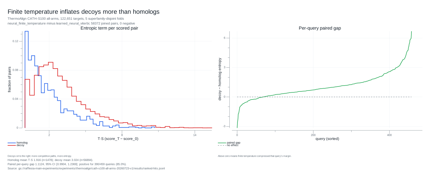
Population	Mean $TS$	n
Homolog pairs	1.916	1,478
Decoy pairs	3.024	56,894

Decoys carry about 1.6x the entropy of homologs. Controlling for query — comparing each query's own homologs against its own decoys, which holds sequence length roughly fixed — the paired gap is 1.1124, 95% CI [0.9904, 1.2369], positive for 390 of 459 queries (85.0%) and positive in all five folds.

So finite temperature is anti-discriminative by construction, and by measurement. The entropy it adds is largest exactly where you least want a score inflated.

We tried to correct for it with a composition- and length-matched null. That arm cost 31.12x fixed Smith-Waterman and still scored below plain Viterbi on nDCG@10 (0.23675 against 0.24420). You cannot cheaply subtract an artifact that is entangled with the quantity you are measuring.

Finding 3: learned energy ties fixed energy, at 15x the cost

Comparison	Recall@100	95% CI	nDCG@10	95% CI
Learned neural − fixed affine SW	−0.00067	[−0.00267, +0.00100]	+0.00101	[−0.00124, +0.00322]

Both intervals straddle zero. The learned neural pair Hamiltonian is statistically tied with a fixed affine Smith-Waterman scorer.

The cost was not tied:

Arm	CPU (ms)	vs fixed SW
Fixed affine Smith-Waterman	1,116,110	1.00x
Learned linear Viterbi	1,112,100	1.00x
Learned neural Viterbi	16,607,028	14.88x
Neural, null-corrected	34,732,955	31.12x

The arm we cannot actually rule on

An attentive reader will have noticed something in the full-scale table that this finding's title glosses over. The learned linear Viterbi posts the highest nDCG@10 of any arm we ran (0.24420 against fixed Smith-Waterman's 0.24316) and the second-highest ROC5 (0.16440 against 0.16220) — at 1.00x cost. The 14.88x penalty belongs to the neural head. The linear head is free.

So why did we keep fixed affine Smith-Waterman?

Not because we measured the linear arm and rejected it. We never ran that paired contrast. Our evidence ledger for this campaign contains four paired comparisons — fixed SW against MaxSim, learned neural against fixed SW, finite temperature against neural Viterbi, and the contact beam against neural Viterbi. There is no paired interval for learned-linear against fixed SW, and the linear arm appears in neither the promoted backbone nor the not-earned list.

Under our own promotion rules an unmeasured contrast cannot promote anything, so the incumbent stays. But we would rather say plainly that the arm which looks best on two point metrics is the arm we have the least evidence about. Those deltas are +0.001 nDCG@10 and +0.002 ROC5 on point estimates whose paired intervals we have not computed; the neural contrast at a comparable magnitude straddled zero comfortably. Our expectation is that the linear arm is another tie. It is an expectation, not a result, and it is the first contrast we would run next.

And the sharpest single measurement in the entire program came from the pair-HMM project. A learned emission head, compared against plain centered cosine at full scale:

Metric	Learned emission − centered cosine
nDCG@10	0
ROC5	0
Recall@100	0
TAP5	−0.0000056

Not "small." Zero. The learned emission model converged onto the inner product.

Three exact zeros invite the obvious objection — that the two arms are the same code path and we measured a bug. They are not, and the shape of the result says why. nDCG@10, ROC5, and Recall@100 are all rank-based: they see only the ordering of results. TAP5 is not — it applies a calibrated score threshold, so it can register a difference in the score values even when the induced ranking is identical. That is exactly the pattern here: the three rank metrics agree to zero, and TAP5 separates the arms at $-5.6\times10^{-6}$. The two scorers emit different numbers; those numbers just sort the same way. A duplicated code path would have driven TAP5 to zero along with everything else.

The pair-HMM project's promotion record reads the same way as the others: ordered inference supported, learned emission head not supported.

Finding 4: predicted structure is not structure

This is the finding that stops the story from being a lazy "simple things win."

Our geometry-transfer experiment ran two arms. Given oracle geometry, the scorer improved with paired ROC5 and nDCG@10 intervals excluding zero — the scorer can genuinely use structural information. Given geometry predicted from sequence by a linear probe, it regressed on every point metric and, in the experiment's own words, behaved like its residue-shuffled control.

The same pattern repeated everywhere we tried to inject predicted structure:

Predicted-structure arm	Result
Embedding contact beam (CATH-S100)	−0.06303 nDCG@10, CI [−0.07683, −0.05009]
Sparse predicted contact graph	R@100 +0.00143 (interval touches zero), ROC5 −0.00171, nDCG@10 −0.00706
Low-rank topology compiler	validation graph F1 +0.000063, against a required 0.01

There is a straightforward reason. Predicted geometry $\hat{g} = f(\text{sequence})$ and the embedding $e = g(\text{sequence})$ are functions of the same input. $\hat{g}$ can only help by making accessible something already implicit in $e$; it introduces no new information. True geometry is a different observable — it comes from the structure, not the sequence — and it measurably helps.

So the correct statement is not that structure is irrelevant to homology. It is that cheap geometry predicted from the same representation is not structure.

That scope matters, and it is worth stating plainly because the obvious counterexample is a good one. Foldseek searches hundreds of millions of AlphaFold-predicted structures and works extremely well — predicted structure clearly can carry homology signal. But an AlphaFold prediction is not what any of our arms used. Ours were a linear probe on ESM2-8M, a sparse contact graph, and a low-rank topology compiler: cheap predictors reading the same single sequence the embedding already read. AlphaFold brings multiple-sequence alignments, which is genuinely additional evidence rather than a re-projection of the same input, and that is precisely the gap the data-processing argument leaves open.

Our result is therefore a statement about cheap same-representation geometry, not about predicted structure in general. Attaching a real structural backend as an independent measurement remains on our roadmap for exactly this reason.

Why this was structurally inevitable

Put the four findings together and a single mechanism explains all of them.

A protein language model is a coarse-graining. Masked-language-model training over protein families produces a representation in which residues that are interchangeable in context receive similar vectors — because interchangeable residues induce similar predictive distributions. That is, definitionally, what a substitution score measures. BLOSUM estimates it by counting substitutions in curated alignments. A pair-HMM emission estimates it by fitting a probabilistic model. ESM2 hands it to you as a geometry, in which the natural pair coupling is an inner product.

If that is true, then $u(i,j) = \langle e_i, f_j \rangle$ is not a crude stand-in for some truer energy that a neural network could refine. It is already the effective pairwise coupling in the coarse-grained coordinates. Fitting an MLP on top is adding higher-order terms to an effective Hamiltonian that has already been diagonalized — which is precisely what a tie at 14.88x looks like, and exactly what an emission head that reproduces cosine to zero difference looks like.

That leaves the question of what the embedding does not encode. It encodes which residues correspond. It does not encode that correspondences must be ordered — that if query residue 10 maps to target residue 40, then query residue 11 cannot map to target residue 12. Order is a global combinatorial constraint over the whole assignment, and no amount of per-residue representation quality supplies it.

Which is why the ordering constraint is the one thing that kept paying, on both benchmarks, in both codebases.

The representation supplies the chemistry. Dynamic programming supplies the order. There is nothing left in between for a learned physical model to do.

Stated as an operational claim: protein alignment over modern embeddings is no longer a thermodynamics problem. It is a combinatorial one. The right algorithm is the zero-temperature ground state of a constrained directed path over a fixed inner-product medium — which is what Smith-Waterman has been since 1981.

What we kept

The retained backbone is unchanged by all of this:

Mango ANN
  -> exact bidirectional salience-weighted MaxSim
  -> fixed embedding affine Smith-Waterman

Relaxation first, because it is cheap and its bound structure makes it a good recall filter. Constrained ground state second, because monotonicity is worth 0.047 nDCG@10 and nothing else we tried was worth anything.

Not earned, and not shipped: the learned neural pair Hamiltonian, finite-temperature ranking, composition-shuffle null ranking, the embedding-derived contact beam, and the learned-value-function alignment accelerator. On a separate ASTRAL95 campaign, free-energy marginalization (2.73x slower), monotone unbalanced optimal transport (2.08x slower), fragment chaining, and domain mosaics all lost to a trained Viterbi with paired intervals excluding zero.

One result there is worth sitting with. The selected ASTRAL95 frontier fused embedding MaxSim with BLOSUM62 Gotoh — a substitution matrix published in 1992 — because the classical lane contributed complementary top-rank signal that none of the learned energy models could. It does not replace the embedding lane; embedding lanes have substantially higher Recall@100. But it earned a place in the fusion, and the neural Hamiltonians did not.

Reproduction

Every number above comes from a durable evidence ledger with a run id, an implementation commit, and published artifacts. We would rather be checked than believed.

Campaign	Run id	Artifacts
CATH-S100 all arms — the full-scale table, Findings 1–3, the CPU ratios, and the frontier-certification ladder	cath-s100-all-arms-20260723-v1 (commit d9fc71edb)	gs://rafflesia-main-experiments/experiments/thermoalign/cath-s100-all-arms-20260723-v1/
Learned pair-HMM, ASTRAL95 — the Viterbi/Forward contrasts and the zero-difference emission head	astral95-learned-pairhmm-q256-k1024-20260723-v1	gs://rafflesia-main-experiments/experiments/pairhmm/astral95-learned-pairhmm-q256-k1024-20260723-v1/
Physics objectives, ASTRAL95 — the learned-objective arms that were not promoted	physics-objectives-astral-20260723-v1 (commit 2bedf133f4)	gs://rafflesia-main-experiments/experiments/softqalign/physics-objectives-astral-20260723-v1/

Each ledger records its own promotion decision, and those decisions are the ones quoted here: ordered_pairhmm_inference: supported, learned_emission_head: not_supported, empirical_significance: not_supported.

What would change our minds

Everything above is conditioned on choices we can name, and each is a way the result could be wrong.

The decisive control is missing, and we know which one it is. Every experiment here varies the scorer while holding the representation fixed. That establishes that learned energy adds nothing on top of ESM2-8M; it does not establish that the representation is why. The experiment that would settle it runs the ladder downward instead: fit the same learned Hamiltonian over deliberately degraded features — one-hot residues, a BLOSUM62 lookup, a smaller or under-trained encoder — and check whether learned energy recovers the value it cannot find on ESM2. If coarse-graining is the mechanism, the gain should appear as the representation degrades and vanish as it improves. If learned energy is flat across that whole range, our explanation is wrong even though the measurements stand. We have not run it, so the mechanism in the previous section is the most economical account of the ties rather than a demonstrated cause.

The encoder is frozen ESM2-8M. Eight million parameters. If the coarse-graining argument is right, the conclusion should strengthen with a larger protein language model — a better representation leaves even less residual structure for a learned energy to capture. But that is a prediction, not a measurement, and a larger model could just as well expose regimes where the inner-product coupling stops being sufficient.

Both benchmarks are structure-derived. CATH-S100 and ASTRAL95 are the right panels for remote homology, but they are not UniRef-scale, and 600 queries against 122,651 targets is not a production corpus.

Some arms were rejected at micro or scout scale. Those stages are designed to reject cheaply and are not permitted to promote. A rejected lane is not a proven-useless lane; it is a lane that did not clear a screening bar.

Our own scaling caveat cuts against over-reading the high-scale numbers. Mango top-2,048 frontiers are certified for every query through 50,000 targets, but for only 33.33% of queries at 100,000 and 17.83% at the full 122,651. Qrel survival falls from 0.939 at 10,000 targets to 0.7937 at 50,000 while every frontier is still certified — so the dominant scaling loss there is not ANN approximation, and it is not the verifier either. Uncertified routing may add further loss at full scale.

That last point is the one we find most interesting, and it sets up the next problem rather than closing this one. The bottleneck is candidate frontier quality and width, followed by MaxSim-to-Smith-Waterman ranking. It is not verifier capacity.

We went looking for a better verifier. The measurements kept telling us the verifier was never the thing that was broken.